3 Machine Learning I

Image source: *Build a Large Language Model (From Scratch)* by Sebastian Raschka

3.1 Machine Learning in a Nutshell

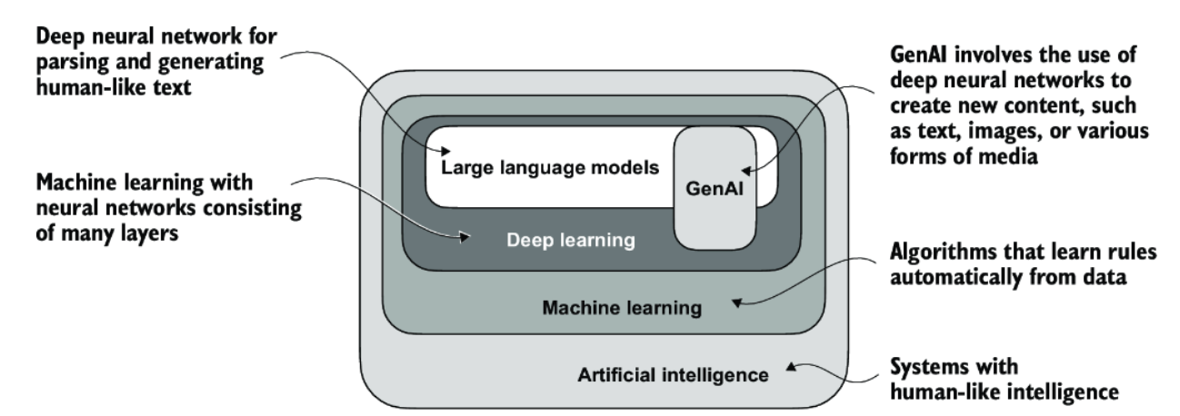
Machine learning is about enabling computers to recognize patterns in data so they can make accurate predictions or decisions without being explicitly programmed for every scenario. At its core, it involves feeding a model real-world examples encoded in a dataset and allowing the computer to learn the relationship between inputs and outputs. Once trained, the model can apply that learned relationship to make predictions on new, unseen data.

To build a machine learning model, we need four key ingredients:

A mathematical model: This defines the form of the mathematical function we’ll use to relate inputs to outputs, for example, a straight line (linear) or a more flexible structure like a neural network (non-linear).

What do we mean by “linear”?

“Linear” in this context means that the effect of $x$ on $\hat{y}$ is proportional and constant: no matter what value of $x$ we choose, an increase of 1 unit in $x$ always increases $\hat{y}$ by exactly $w_1$ units. This property makes the model highly interpretable.

Training data: A collection of real-world examples that pair inputs with their corresponding outputs. The quality and relevance of this data are crucial to how well the model can learn and make accurate predictions.
A “loss” function: A mathematical expression that measures how far off the model’s predictions are from the correct answers. It provides feedback to help the model improve over time.
A training algorithm: A step-by-step procedure that combines the first three ingredients in a way that minimizes the prediction errors produced by the model. This is where the so-called learning takes place.

There are many business use cases for machine learning, a few of which are listed below. We’ll start with the simplest possible machine learning model: simple linear regression. It’s a powerful tool that helps us understand the core ideas behind more complex models, including the ones that power today’s cutting-edge AI systems like ChatGPT and several of the examples in the table below.

Use Case	Sample Inputs	What does the model output?	What Business Question is Being Answered?
Price Prediction	Property size, location, features	Numeric price estimate	How should I price products to stay competitive and profitable?
Demand Forecasting	Historical sales, promotions, holidays	Predicted sales volume	How can I manage inventory or staffing to meet demand?
Credit Risk Scoring	Income, credit history, employment data	Risk category (e.g., low/medium/high)	Should I approve this loan, and at what interest rate?
Email Spam Detection	Email content, sender info, subject line	Binary label: spam or not spam	How can I prevent unwanted emails from reaching users’ inboxes?
Sentiment Analysis	Review text, social media posts	Sentiment label (positive/negative)	What is the public opinion about my product or brand?
Disease Diagnosis	Symptoms, test results, demographics	Disease class (e.g., flu, COVID, none)	How can I assist doctors in making accurate and timely diagnoses?
Energy Usage Estimation	Time of day, weather, appliance usage	Predicted energy consumption	How should I manage power supply or optimize grid efficiency?

3.2 Simple Linear Regression

3.2.1 1st Ingredient: Mathematical model

A simple linear regression model takes a single input variable $x$ and predicts the value of a corresponding output variable $y$. For example, the input variable might represent a house’s square footage, and the output variable could represent the value of the home.

We can write down the relationship between square footage and value in the form of a mathematical equation (also called a mathematical function or a model):

\[ y = w_0 + w_1 x \]

Where $y$ represents the home value and $x$ represents the square footage.

In machine learning jargon $w_0$ and $w_1$ are called the parameters or weights of the model (hence the use of $w$ in the notation) and describe the nature of the relationship between $x$ and $y$. $w_0$ and $w_1$ are the numbers that the computer will learn (i.e. derive) based on what is observed in real life which will be encoded into training data discussed in the next section.

In other fields such as econometrics the weights (also called coefficients) might be introduced using the Greek alphabet notation of $\alpha$ and $\beta$.

Simple linear regression might bring to mind the equation of a line in slope-intercept which is often presented as:

\[ y = mx + b \]

where $x$ and $y$ are numbers in the coordinate plane with $m$ representing the slope of the line and $b$ representing the y-intercept (the point where the line crosses the y-axis) as shown in the image below:

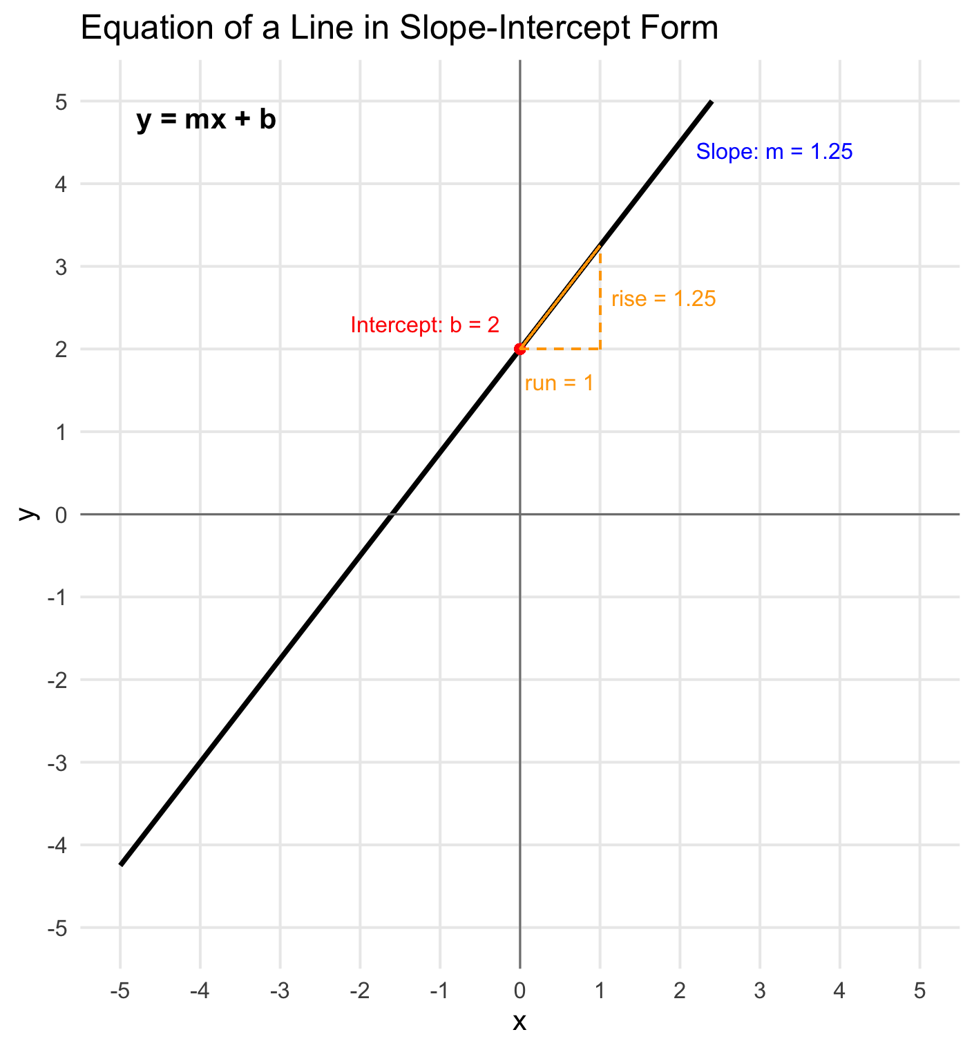
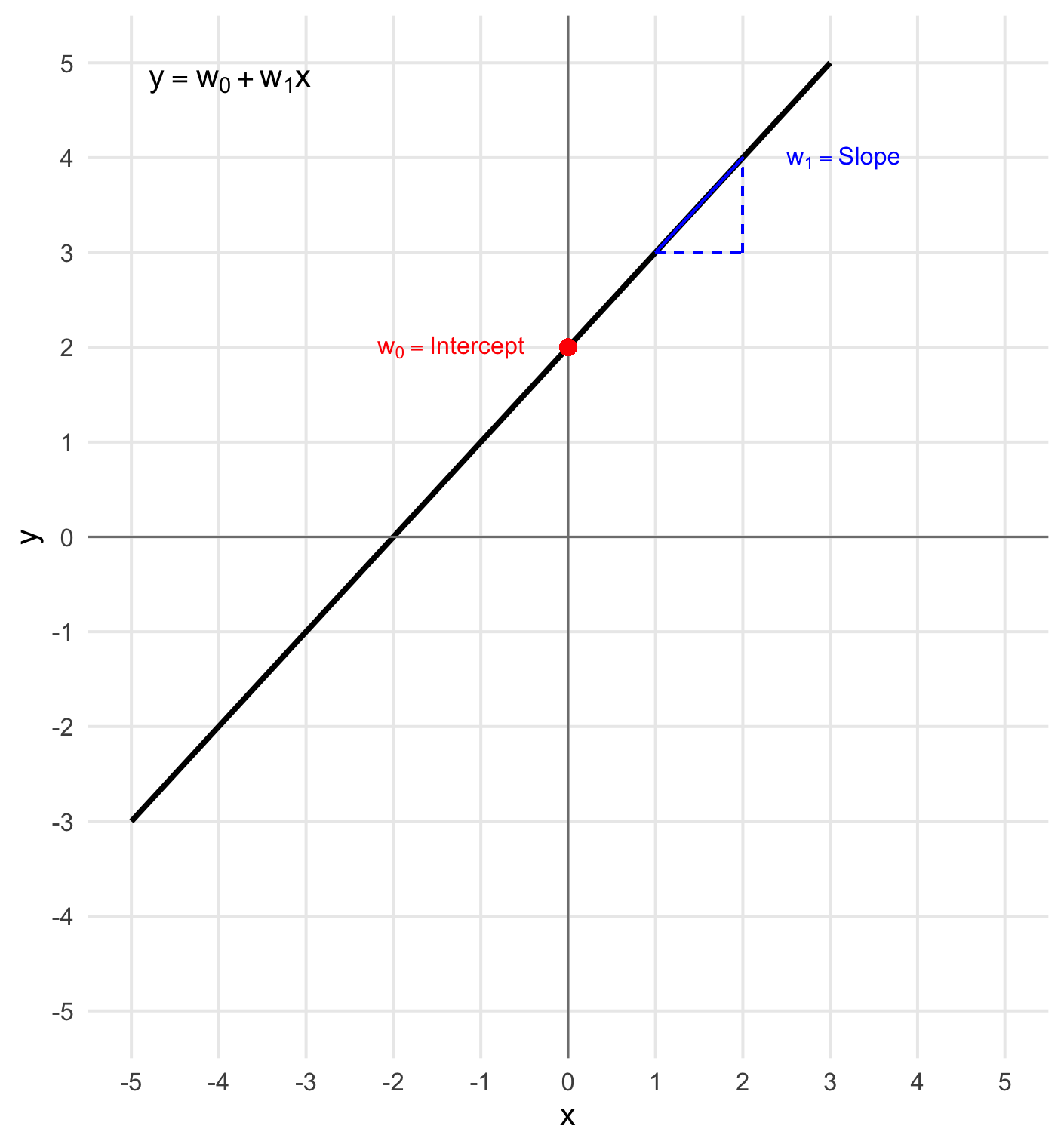
Simple linear regression and the equation of a line are in fact the same mathematical equation. In the context of linear regression, we simply use different notation: $w_1 = m$ (the slope), and $w_0 = b$ (the y-intercept which in machine learning is referred to as the bias term).

It’s common for different fields of study to use different notation and words for the same mathematical concepts. Unfortunately this can be one of the biggest sources of confusion for students so we will make an effort to call out these differences throughout the course.

Now that we’ve shown that simple linear regression is actually just the equation of a line where $w_0$ is the y-intercept and $w_1$ is the slope we can have a visual picture in mind for how an input variable $x$ and the output variable $y$ are related.

Intuition check

Think about our home value example, where we’re predicting a house’s price based on its square footage.

What does your intuition tell you about the values $w_0$ and $w_1$ are likely to take on once they are estimated?
Do you expect them to be positive or negative numbers?
Assume $x$ was $0$, what would the equation be telling you?

As soon as we come up with values for $w_0$ and $w_1$ have a way predicting values of $y$ when plugging in any value of $x$ to the fitted equation.

The goal of machine learning is to learn the best possible values $w_0$ and $w_1$ allowing us to make good predictions of a homes value based on it’s square footage. We will soon explore how the computer learns these weight values but to build our intuiton on what the model does we can start by simply guessing values for the weights. For example, let’s assume:

\[ w_0 = 50,\!000 \quad \text{and} \quad w_1 = 200 \]

Then our function becomes:

\[ \hat{y} = 50,\!000 + 200x \]

We use the notation $\hat{y}$ (read as “y-hat”) here to emphasize that this is a now predicted value based on the model, not an observed or actual value.

This act of using the trained model to compute a prediction based on an input $x$ is also called inference since we are inferring an estimated output $\hat{y}$.

Using this model we can predict that a home with 3,000 square feet will have a value of:

\[ \hat{y} = 50,\!000 + 200 \cdot 3,\!000 = \$650,\!000 \]

Now, consider what the model predicts for a home with 0 square feet:

\[ \hat{y} = 50,\!000 + 200 \cdot 0 = \$50,\!000 \]

This implies that the base value of the property—the land alone, with no house—might be interpreted as $50,000. This is exactly why both $w_0$ and $w_1$ are necessary. If we had included only $w_1 x$ and omitted $w_0$, the model would always predict 0 for an input of $x = 0$, which might not reflect the reality (e.g., land still has value).

In machine learning, the term bias is used to refer to this $w_0$ value. The name comes from the fact that it shifts (or “biases”) the entire output of the model up or down, independent of the input. Geometrically, it determines the $y$-intercept of the prediction line. It allows the model to better fit real-world data.

Choosing a different set of weight values would result in a different equation, resulting in a different prediction. For example, assume instead that $w_0 = 25,000$ and $w_1 = 300$ resulting in the following equation:

\[ \hat{y} = 25,000 + 300 x \]

This model would predict that the same 3,000 square-foot home has a much higher value of $\$925,000 = 25,000+300*3,000$.

Let’s assume the $3,000 square foot home we have in mind recently sold for $800,000 reflecting it’s true value (a single instance of $y$). We could then compute the error associated with each set of model weights as the absolute value of the prediction error as follows:

Prediction error when $w_0 = 50,\!000$ and $w_1 = 200$: $\left| 650,000 - 8000000 \right| = 150,000$
Prediction error when $w_0 = 25,\!000$ and $w_1 = 300$: $\left| 925,000 - 8000000 \right| = 125,000$

Given these results we might reasonably conclude that the second set of model weights produced the better prediction, since it was less wrong by $25,000.

In machine learning this prediction error is commonly called the model’s loss, that is, how far off the prediction is from the observed truth. The mathematical function by which we compute prediction error is called the loss function. In our case, we could represent our choice of loss function as $\left| \hat{y} - y \right|$.

There are many possible choices of loss function. For example, we didn’t have to use absolute value, we could have simply taken the difference as our measurement of loss. We will discuss loss functions and introduce the most commonly used loss functions in later sections.

3.2.2 2nd Ingredient: Training Data

In order for a computer to learn the best weight values for a model, we need to communicate with it in the language it understands: data. In this context, “data” refers to numerical values organized in rows and columns, like a spreadsheet or matrix. Each row is a single example, and each column holds a particular feature or label.

For our home value prediction example, imagine a simple dataset with two columns:

One column for the square footage of a home (the input), and
One column for the value of the home (the output).

Each row contains both the square footage and the corresponding value for a particular house. Together, each pair of values forms what we call an input-output pair. A complete set of these pairs is called a dataset.

We can write this dataset using the following compact mathematical notation:

\[ \{(x^{(i)}, y^{(i)})\}_{i=1}^n \]

This might look intimidating at first, but it’s just a convenient way of saying:

“We have $n$ examples. For each example $i$, we observe an input $x^{(i)}$ and a corresponding output $y^{(i)}$.”

Let’s break down the notation a bit further:

The curly braces $\{ \}$ mean we’re describing a set, a collection of items.
The superscript $(i)$ just means “for example number $i$”
Each item in the set is a pair: $(x^{(i)}, y^{(i)})$ where:
- $x^{(i)}$ is the input (e.g., square footage) for the $i$th example
- $y^{(i)}$ is the output (e.g., home value) for that same example
The subscript $_{i=1}^n$ tells us there are $n$ examples and we are referring to all $1$ to $n$ of them.

If you wrote this out as a table, it might look like this:

Example ($i$)	$x^{(i)}$ = Square Footage	$y^{(i)}$ = Home Value
1	1200	250,000
2	1400	275,000
3	1600	300,000
…	…	…
$n$	(last example)

This is the kind of data we use to “train” a machine learning model, by showing it many examples, we give it a chance to learn the relationship between inputs and outputs.

Terminology: Inputs and Outputs

In different fields and contexts, we often use different terms for the same underlying ideas. Here’s a helpful reference for the various names used for inputs and outputs in machine learning and related areas:

Concept	Common Synonyms	Notes
Input	Feature, Independent Variable, Predictor, Covariate, Regressor, $x$	The value(s) we feed into the model to make a prediction. Can be one variable or many.
Output	Label, Target, Dependent Variable, Response, $y$	The value the model is trying to predict or learn from.
Input-Output Pair	Example, Observation, Data Point, $(x^{(i)}, y^{(i)})$	A single row of data showing both the input and the correct output.
Collection of Examples	Dataset, Training Data, Sample	All the input-output pairs we give to the model to learn from.
Predicted Output	Prediction, Estimate, $\hat{y}$	The output the model thinks is correct, based on what it learned.

There are actually four equivalent ways of representing a dataset, each useful in different contexts. You will be greatly aided in your study of machine learning if you can recognize and switch between all four forms with ease. Different textbooks, courses, tutorials and code libraries will use different representations so developing fluency in all of them will help you understand ideas more deeply and communicate more clearly.

Mathematical Set Notation:

This is the notation we just introduced:

\[ \{(x^{(i)}, y^{(i)})\}_{i=1}^n \]

It represents the dataset as a collection of $n$ input-output pairs, where each $x^{(i)}$ is an input and each $y^{(i)}$ is the corresponding output. This form is widely used in textbooks and research papers because of its compactness and precision. It’s the language of mathematics, and it’s especially helpful when trying to understand what’s happening under the hood as computer code executes. By using this notation, we can reason more clearly about how models learn and make predictions.

Spreadsheet or Table Format:

This is the most familiar form for most people and is often used in business and statistics. Each row represents an example; each column represents a variable or feature.

Example ($i$)	$x^{(i)}$ = Input (e.g., SqFt)	$y^{(i)}$ = Output (e.g., Price)
1	1200	250,000
2	1400	275,000
3	1600	300,000
…	…	…
$n$	—	—

This is also the format used in tools like Excel, Google Sheets, or data frames in Python and R.

Mathematical Matrix Notation:

Matrix notation is a compact and powerful way to represent datasets and linear regression models. It helps us generalize models to many inputs and use efficient numerical libraries for computation.

In matrix form, a simple linear regression with one input variable looks like this:

\[ \hat{y} = \begin{bmatrix} 1 & x \end{bmatrix} \begin{bmatrix} w_0 \\ w_1 \end{bmatrix} = w_0 + w_1 x. \]

Here:

The “1” in the input vector allows us to represent the intercept term $w_0$ together with the slope $w_1$.
This convention turns the model into a dot product (vector multiplication).

While this may initially feel like a notational trick, it is a standard approach in regression modeling and is essential for applying matrix operations efficiently.

This notation extends naturally to represent the entire training dataset. When including an intercept, we create an input matrix (also called a design matrix) by adding a column of ones on the left:

\[ \mathbf{X} = \begin{bmatrix} 1 & x^{(1)} \\ 1 & x^{(2)} \\ \vdots & \vdots \\ 1 & x^{(n)} \end{bmatrix}, \] More generally:

The design matrix $\mathbf{X}$ has shape $(n, d + 1)$, where:
- $n$ = number of training examples (rows).
- $d$ = number of input features.
- The extra column of ones accounts for the intercept (also called the bias term).

If we have more than one input feature (for example, square footage and number of bedrooms, etc), $\mathbf{X}$ becomes:

\[ \begin{bmatrix} 1 & x_1^{(1)} & x_2^{(1)} & \cdots & x_d^{(1)} \\ 1 & x_1^{(2)} & x_2^{(2)} & \cdots & x_d^{(2)} \\ \vdots & \vdots & \vdots & \ddots & \vdots \\ 1 & x_1^{(n)} & x_2^{(n)} & \cdots & x_d^{(n)} \end{bmatrix} \]

The output vector $\hat{\mathbf{y}}$ stores the predicted values (e.g., house prices):

\[ y = \begin{bmatrix} y^{(1)} \\ y^{(2)} \\ \vdots \\ y^{(n)} \end{bmatrix} \]

The weight vector $\mathbf{w}$ stores the weight parameters:

\[ \mathbf{w} = \begin{bmatrix} w_0 \\ w_1 \\ \vdots \\ w_{d} \end{bmatrix} \] This leads to the compact matrix equation for all predictions:

\[ \hat{\mathbf{y}} = \mathbf{X} \mathbf{w} = \begin{bmatrix} 1 & x_1^{(1)} & x_2^{(1)} & \cdots & x_d^{(1)} \\ 1 & x_1^{(2)} & x_2^{(2)} & \cdots & x_d^{(2)} \\ \vdots & \vdots & \vdots & \ddots & \vdots \\ 1 & x_1^{(n)} & x_2^{(n)} & \cdots & x_d^{(n)} \end{bmatrix} \begin{bmatrix} w_0 \\ w_1 \\ w_2 \\ \vdots \\ w_d \end{bmatrix} \] > Matrix notation helps us express models clearly and allows computers to compute predictions for all examples at once. This approach is essential when scaling to many features and large datasets. We will rely on this notation throughout the course.

Code Representation (Arrays or Tensors):
When implementing models in code, we typically use arrays (Python’s NumPy package) or tensors (Python’s PyTorch package) which are data structures that store values in memory for numerical computation.

Below is an example with NumPy

# NumPy
import numpy as np
X = np.array([[1200], [1400], [1600]])
y = np.array([[250000], [275000], [300000]])
print("X =", X)
print("y = ", y)

X = [[1200]
 [1400]
 [1600]]
y =  [[250000]
 [275000]
 [300000]]

So what does this mean?

X is a matrix of inputs (in this case, just one feature: square footage).
Each row represents one example:
- 1200 square feet
- 1400 square feet
- 1600 square feet
y is a vector of outputs (the target values, like home prices).
Each row in y matches the corresponding row in X.

Let’s now connect this code back to the set and matrix representations of a dataset.

Equivalence with Set Notation

In set notation this tiny dataset could be represented as three input-output pairs:

\[ \{(x^{(i)}, y^{(i)})\}_{i=1}^3 \] More specifically:

$x^{(1)} = 1200$, $y^{(1)} = 250{,}000$
$x^{(2)} = 1400$, $y^{(2)} = 275{,}000$
$x^{(3)} = 1600$, $y^{(3)} = 300{,}000$

Each pair $(x^{(i)}, y^{(i)})$ is represented by a row in X and the corresponding row in y.

Equivalence with Matrix Notation

We can also see how this toy dataset would be written in matrix notation as a pair of matrices, one for the inputs and one for the outputs:

\[ X = \begin{bmatrix} x_1^{(1)} \\ x_1^{(2)} \\ x_1^{(3)} \end{bmatrix} = \begin{bmatrix} 1200 \\ 1400 \\ 1600 \end{bmatrix}, \quad y = \begin{bmatrix} y^{(1)} \\ y^{(2)} \\ y^{(3)} \end{bmatrix} = \begin{bmatrix} 250{,}000 \\ 275{,}000 \\ 300{,}000 \end{bmatrix} \]

$X$ is an $n \times 1$ input matrix (with one feature per example),
$y$ is an $n \times 1$ output vector (with one label per example).

PyTorch Example

Lastly, below we represent the same toy dataset using PyTorch, currently the most popular deep learning library, and the one used to develop many modern large language models (LLMs).

PyTorch uses a data structure called a tensor.

A tensor is a generalization of familiar objects like scalars, vectors, and matrices:

A scalar is a 0-dimensional tensor (e.g., 5)
A vector is a 1-dimensional tensor (e.g., [1200, 1400, 1600])
A matrix is a 2-dimensional tensor (e.g., a table of numbers)
A 3D tensor is a collection or stack of matrices. You can think of it as a book of matrices, where each page is a 2D grid (matrix), and the whole book has depth (i.e., the number of pages)
A 4D tensor is a collection of 3D tensors. You can think of it as a library of books, where:
- Each book is a 3D tensor (a stack of matrices),
- Each page in a book is a matrix,
- And each matrix contains rows and columns of numbers.

Increasing the tensor dimension allows us to compactly describe multiple sets of structured data and for a computer to perform parallel computations efficiently which is essential when training modern LLMs.

In theory, there is no limit on the number of dimensions a tensor can have.

In practice, we won’t need more than 4D tensors to build modern large language models (LLMs).

For simple models like linear regression, a 2D tensor (i.e., a matrix) is sufficient to represent the data.

Below we illustrate the same toy data set using a PyTorch tensor.

import torch

# Input data: square footage (in one column)
X = torch.tensor([[1200.], [1400.], [1600.]])

# Output data: home prices
y = torch.tensor([[250000.], [275000.], [300000.]])

print("X (inputs):")
print(X)

print("\ny (outputs):")
print(y)

X (inputs):
tensor([[1200.],
        [1400.],
        [1600.]])

y (outputs):
tensor([[250000.],
        [275000.],
        [300000.]])

The dot (.) at the end of the numbers (like 1200. or 250000.) indicates that the numbers are being treated as floating point numbers (i.e., float type) rather than integers. A floating point number is a number that can represent decimal values on a computer, in contrast to an integer, which can only represent whole numbers. PyTorch models expect inputs and outputs to be floating point numbers because most model operations involve decimals.

We will soon use a set of training Data to help learn model parameters but before doing so we need to introduce the remaining two ingredients for machine learning: loss functions and training algorithms.

3.2.3 3rd Ingredient: Loss Function

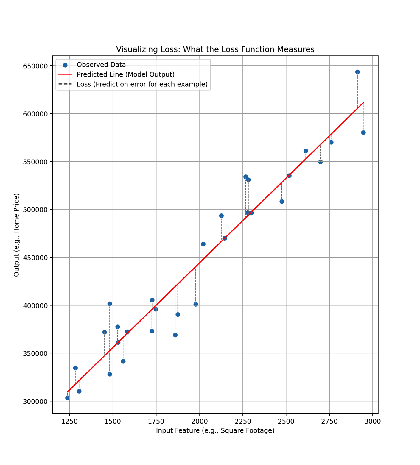
A loss function is separate mathematical equation whose purpose it to quantify the error between a model’s predictions $\hat{y}^{(i)}$ and the true output values observed in the training data $y^{(i)}$. When discussing mathematical model structure (i.e. simple linear regression), we briefly introduced the notion of a loss function and used the absolute value of the difference between $\hat{y}^{(i)}$ and between and $y^{(i)}$ to measure prediction error (i.e. loss): $\left| \hat{y} - y \right|$. Note that this loss is calculated for each individual training example. That is, if we had 100 training examples (i.e. rows of data) containing the square footage and home value for 100 homes, we could compute the loss for each of these examples. The dotted lines in the plot below help you visualize the loss for each example in a set of training data.

We could then find the average loss by summing up the observation level loss and dividing by the number of observations to get what is commonly called Mean Absolute Error (MAE), written as:

\[ \frac{1}{n} \sum_{i=1}^{n} \left| \hat{y}^{(i)} - y^{(i)} \right| \]

MAE is an intuitive choice for a loss function, but not the only choice. There are other equations that will measure prediction error in slightly different ways. One such equation and the most commonly used loss function when learning parameters for a simple linear regression is called Mean Squared Error (MSE), written as:

\[ \frac{1}{n} \sum_{i=1}^{n} \left( \hat{y}^{(i)} - y^{(i)} \right)^2 \]

Recall that $\hat{y} = w_0 + w_1 x$ hence we can plug $w_0 + w_1 x$ into the equation for $\hat{y}$ to make clear that the loss function, which we denote as $\mathcal{L}$ (a stylized version of the capital Latin letter L), is a function of two variables: $w_0$ and $w_1$. This means that different values of $w_0$ or $w_1$ or both will yield different loss values. The goal of machine learning is to find (i.e. learn) the values of $w_0$ and $w_1$ that will make this loss function (i.e., total prediction error) as small as possible.

\[ \mathcal{L}(w_0, w_1) = \frac{1}{n} \sum_{i=1}^n (\hat{y}^{(i)} - y^{(i)})^2 = \frac{1}{n} \sum_{i=1}^n (w_0 + w_1 x^{(i)} - y^{(i)})^2 \]

In the next section, we will introduce a training algorithm called gradient descent. This algorithm systematically searches through different combinations of values for $w_0$ and $w_1$ to find those that minimize the loss or in other words, to learn the best-fitting line.

To really understand how gradient descent works, we first need to deepen our understanding of the loss function, specifically how it behaves with respect to the parameters $w_0$ and $w_1$.

Recall that in simple linear regression, we model predictions as:

\[ \hat{y} = w_0 + w_1 x \]

When we think of this as a function of the input variable $x$, we can plot it as a straight line on a 2D coordinate system (with $x$ on the horizontal axis and $\hat{y}$ on the vertical axis) as we did earlier.

But now, let’s flip our perspective. In the previous section, we learned that training data consists of actual examples, pairs of $x$ and $y$, from the real world. So once we have a training dataset, $x$ and $y$ are known. That means we no longer need to treat $x$ as a variable in our model equation.

In this case, the prediction formula:

\[ \hat{y} = w_0 + w_1 x \]

becomes a function where $w_0$ and $w_1$ are the unknown variables. Our goal is to adjust these weights to reduce the difference between our predicted values $\hat{y}$ and the actual outcomes $y$. So during model training, we treat $w_0$ and $w_1$ as the variables to solve for, which turns our loss function into a function of two variables, $w_0$ and $w_1$:

\[ \mathcal{L}(w_0, w_1) = \frac{1}{n} \sum_{i=1}^n (\hat{y}^{(i)} - y^{(i)})^2 = \frac{1}{n} \sum_{i=1}^n (w_0 + w_1 x^{(i)} - y^{(i)})^2 \] Don’t be intimidated by the notation. Once we have a training dataset, all the $x^{(i)}$ and $y^{(i)}$ values are known values. The only unknowns we are solving for are $w_0$ and $w_1$.

Unpacking the notation of the MSE Loss Function

This is called the Mean Squared Error (MSE) loss function, and it helps us measure how good or bad our model’s predictions are.

The big curly $\mathcal{L}$ is a stylized version of the capital Latin letter L. In this context, $\mathcal{L}$ stands for “Loss” or sometimes “Loss function.”

$w_0$ and $w_1$ are the parameters (or weights) of our simple linear regression model. Notice that they are playing the roles of unknown variables in this notation: $\mathcal{L}(w_0, w_1)$. This is because we don’t know what these values are or should be yet, that’s what we want the computer learn for us.
$x^{(i)}$ is the input (e.g., square footage of a house)
$\hat{y}^{(i)} = w_0 + w_1 x^{(i)}$ is the model’s predicted output (e.g., the predicted house price).
$y^{(i)}$ is the true value (the actual house price for data point $i$).
$(\hat{y}^{(i)} - y^{(i)})^2$ is the squared error: how far off the prediction is, squared to make sure it’s always positive and to penalize big mistakes more than small ones.
$\sum_{i=1}^n$ adds up the squared errors for all $n$ data points in our dataset (the Greek letter $\sum$ is called “capital sigma” and means we should “add up a bunch of terms”)
$\frac{1}{n}$ takes the average of all those squared error terms.

This function tells us how well our model is performing overall. A smaller value means our predictions on average are close to the true values, and a larger value means on average we’re making bigger mistakes.

Our goal is to find the values of $w_0$ and $w_1$ that make this loss function as small as possible.

Because the loss depends on both $w_0$ and $w_1$, we need three dimensions to visualize and plot this function:

One axis for $w_0$
One axis for $w_1$
A vertical axis for the loss value $\mathcal{L}$ (often labeled the $z$-axis in other contexts)

As the saying goes, a picture is worth a thousand words, so let’s visualize what this looks like.

In the plot below, we graph the loss function $\mathcal{L}(w_0, w_1)$ to see it as a 3D surface, with $w_0$ on the x-axis, $w_1$ on the y-axis, and the height of the surface representing the mean squared error loss $\mathcal{L}$. This gives us a landscape of possible values of $w_0$ and $w_1$ to choose from.

The plot also includes contour lines, which are like the topographical lines you see on a map. These contours help you visualize the height of the surface even when looking down from above onto the flat 2D plane. The contour lines will be especially helpful in the next section when we explore how adjusting the weights changes the loss value.

MSE Loss Surface with Contours

As can be seen from the plot, there are many possible choices of $w_0$ and $w_1$, each resulting in a different loss value. In the next section, we will study a foundational algorithm called gradient descent which is designed to intelligently and iteratively explore different combinations of $w_0$ and $w_1$, calculating the loss that results from each combination. The process continues until convergence occurs, that is, until the algorithm believes it has found the best choice of weights that minimize the loss. We’ll explore the details of how gradient descent works in the next section.

Intuition Check

Which choice of weight values is better: point A or point B? Why?

Why use MSE for the loss function?

MSE is the most commonly used loss function for regression problems because it has several useful properties:

Smooth and differentiable: The squaring operation makes the MSE function smooth and continuous, which is important for optimization methods like gradient descent that rely on computing derivatives. (discussed in the next section)
Penalizes large errors: By squaring the difference between prediction and truth, MSE emphasizes larger errors more than smaller ones. This is often desirable when big mistakes are especially costly.
Unique minimum: For linear models, the MSE loss function is convex (it’s bowl shaped), meaning it has a single global minimum. This makes optimization straightforward and ensures reliable convergence during training.

These properties make MSE both practical and theoretically sound for training models to make accurate predictions.

3.2.4 4th Ingredient: Training Algorithm

Once we’ve selected a loss function, the next challenge is figuring out how to minimize it, that is, how to find the values of $w_0$ and $w_1$ that make the loss as small as possible.

To build intuition, imagine you’re standing somewhere on the inside of a smooth, canyon-shaped surface like the 3D plot shown in the last section. This surface represents the loss function, and your location corresponds to a specific pair of weights: $(w_0, w_1)$. Your goal is to hike down to the very bottom of the canyon, the point where the loss is lowest and your model makes its best predictions.

But how do you know which way to step?

This is where the training algorithm called gradient descent comes in. It uses the concept of a derivative (a rate of change from calculus) to calculate the slope of the loss surface at your current position. Then it suggests a small step in the direction that will reduce the loss the fastest: the steepest descent.

It’s called an algorithm because it repeats this process: take a step, recalculate the slope, take another step while gradually working its way toward the minimum.

In this way, gradient descent acts like a smart compass that always points you downhill in the direction that leads most quickly to better predictions.

That explains what descent means in gradient descent, but what about gradient?

Gradient is just a fancy word for the direction of steepest ascent (what we’d call the slope in single variable calculus). Since we want to go downhill, toward lower loss, we will actually move in the opposite (i.e. negative) direction of the gradient, hence the name gradient descent.

Since we are working with a loss function of two variables (the weights), $\mathcal{L}(w_0, w_1)$, there are two directions in play for each step we take down the hill. In this case, the gradient is a vector with two components, each representing the rate of change of the loss with respect to one of the weights (you can think of each component as the “slope” in a particular direction). Mathematically, these components are written as:

$\frac{\partial \mathcal{L}}{\partial w_0}$: how the loss changes when we adjust $w_0$ $\frac{\partial \mathcal{L}}{\partial w_1}$: how the loss changes when we adjust $w_1$

Together, these two components form the gradient vector of the loss function.

This is written using the nabla symbol $\nabla$ (pronounced “nabla”, named after an ancient harp), which represents the gradient operator:

\[ \nabla \mathcal{L}(w_0, w_1) = \begin{bmatrix} \frac{\partial \mathcal{L}}{\partial w_0} \\ \frac{\partial \mathcal{L}}{\partial w_1} \end{bmatrix} \]

The notation looks intimidating, but let’s break it down symbol by symbol:

$\nabla$ is a mathematical operator implying an action is being taken, in this case, computing a series of partial derivatives with respect to each weight
The partial derivative symbol $\partial$ (pronounced “partial”) means we’re measuring the rate of change of the loss $\mathcal{L}$ with respect to just one variable $w_0$ or $w_0$, keeping the other constant.
$\mathcal{L}$ (script L) represents the loss function, which tells us how far off our model’s predictions are from the actual outcomes.
$w_0$ and $w_1$ are the parameters of our model.
$\begin{bmatrix}\end{bmatrix}$ combines all components into a single vector

Just like other more familiar mathematical operators, such as addition $+$ and multiplication $\times$, the $\nabla$ operator means we will perform some operation on whatever equation or numbers we are applying to. In our case, we are taking the partial derivatives of the loss function with respect to each weight in order to obtain the gradient vector. Below, we will show how the partial derivitives of the loss function using rules from calculus.

What is a derivative?

A derivative is a way of measuring how fast something is changing.

In simple terms, the derivative tells you the slope of a function at a specific point—that is, how steep the function is at that spot.

Imagine this:

You’re walking up a hill, and you want to know how steep it is right where you’re standing. That steepness, the instantaneous slope, is the derivative.

If the slope is positive, you’re going uphill.
If the slope is negative, you’re going downhill.
If the slope is zero, you’re on flat ground (maybe the top or bottom of the hill).

Mathematically:

If $f(x) = x^2$, then the derivative is:

\[ \frac{df}{dx} = 2x \]

At $x = 3$, the slope is $2 \cdot 3 = 6$, so the curve is rising steeply.

In gradient descent, we’re just following the steepest slope as we hike downhill toward the lowest point.

What is a partial derivative?

A partial derivative is just the derivative of a multivariable function with respect to one variable at a time, while holding all the other variables constant.

Think of it like asking:
> “If I only adjust this one knob (say, $w_0$), how does the output change, assuming all other knobs stay fixed?”

Example:

Suppose we have this function with two variables:

\[ f(w_0, w_1) = w_0^2 + 3w_0 w_1 + w_1^2 \]

We can take the partial derivatives:

With respect to $w_0$: \[ \frac{\partial f}{\partial w_0} = 2w_0 + 3w_1 \]
With respect to $w_1$:

\[ \frac{\partial f}{\partial w_1} = 3w_0 + 2w_1 \]

Each tells us how the function changes in that direction, treating the other variable like a constant.

This is essential for gradient descent: we compute the slope in each direction (each weight), then use those partials to form the gradient vector.

Recall that our mean squared error (MSE) loss function is:

\[ \mathcal{L}(w_0, w_1) = \frac{1}{n} \sum_{i=1}^n (\hat{y}^{(i)} - y^{(i)})^2 = \frac{1}{n} \sum_{i=1}^n (w_0 + w_1 x^{(i)} - y^{(i)})^2 \] To take the partial derivatives we apply the chain rule which gives us:

What is the Chain Rule

The chain rule is a way to take the derivative of a function inside another function.

Think of it like peeling an onion: you take the derivative of the outer layer, then multiply it by the derivative of the inner layer.

Example:

Suppose you have:

\[ f(x) = (3x + 1)^2 \]

This is a composition of two functions:

Outer function: $u^2$
Inner function: $u = 3x + 1$

Using the chain rule:

\[ \frac{df}{dx} = \frac{d}{du}(u^2) \cdot \frac{du}{dx} = 2u \cdot 3 = 2(3x + 1) \cdot 3 = 6(3x + 1) \]

So even though the original function looks complicated, we can compute the derivative one layer at a time and then multiply the results from each layer.

This same principle is applied to find the partial derivatives of a loss function like MSE.

Partial Derivative with respect to $w_0$

\[ \frac{\partial \mathcal{L}}{\partial w_0} = \frac{2}{n} \sum_{i=1}^n (w_0 + w_1 x^{(i)} - y^{(i)}) \times 1 = \frac{2}{n} \sum_{i=1}^n (w_0 + w_1 x^{(i)} - y^{(i)}) \]

Partial Derivative with respect to $w_1$

\[ \frac{\partial \mathcal{L}}{\partial w_1} = \frac{2}{n} \sum_{i=1}^n (w_0 + w_1 x^{(i)} - y^{(i)}) \times x^{(i)} \]

Putting the two partial derivtives into a vector gives us the gradient of the loss function:

\[ \nabla \mathcal{L}(w_0, w_1) = \begin{bmatrix} \frac{\partial \mathcal{L}}{\partial w_0} \\ \frac{\partial \mathcal{L}}{\partial w_1} \end{bmatrix} = \frac{2}{n} \sum_{i=1}^n \begin{bmatrix} w_0 + w_1 x^{(i)} - y^{(i)} \\ (w_0 + w_1 x^{(i)} - y^{(i)}) \cdot x^{(i)} \end{bmatrix} \] Don’t lose sight of the fact that this apparently complex notation just represents simple numbers in the end.

For example, let’s assume our training data was:

$x^{(1)} = 0, \; y^{(1)} = 1$
$x^{(2)} = 1, \; y^{(2)} = 3$
$x^{(3)} = 2, \; y^{(3)} = 5$
$x^{(4)} = 3, \; y^{(4)} = 7$

With initial weights of: $w_0 = 1, \; w_1 = 1$

Then, substituting all these values into the gradient equation above we get:

\[ \begin{align*} &= \frac{2}{4} \Bigg( \begin{bmatrix} 1 + 1 \cdot 0 - 1 \\ (1 + 1 \cdot 0 - 1) \cdot 0 \end{bmatrix} + \begin{bmatrix} 1 + 1 \cdot 1 - 3 \\ (1 + 1 \cdot 1 - 3) \cdot 1 \end{bmatrix} + \begin{bmatrix} 1 + 1 \cdot 2 - 5 \\ (1 + 1 \cdot 2 - 5) \cdot 2 \end{bmatrix} + \begin{bmatrix} 1 + 1 \cdot 3 - 7 \\ (1 + 1 \cdot 3 - 7) \cdot 3 \end{bmatrix} \Bigg) \\ &= \frac{2}{4} \left( \begin{bmatrix} 0 \\ 0 \end{bmatrix} + \begin{bmatrix} -1 \\ -1 \end{bmatrix} + \begin{bmatrix} -2 \\ -4 \end{bmatrix} + \begin{bmatrix} -3 \\ -9 \end{bmatrix} \right) \\ &= \frac{2}{4} \begin{bmatrix} -6 \\ -14 \end{bmatrix} \\ &= \begin{bmatrix} -3 \\ -7 \end{bmatrix} \end{align*} \]

So the negative gradient of the loss function calculated at:

\[ \begin{bmatrix}w_0 \\ w_1 \end{bmatrix} = \begin{bmatrix} 1 \\ 1 \end{bmatrix} \]
is:

\[ \nabla \mathcal{L}(w_0, w_1) = \begin{bmatrix} 3 \\ 7 \end{bmatrix} \]

The weight vector and the gradient vector always have the same number of components because the gradient is composed of the partial derivatives with respect to each weight, one for every weight parameter.

Our goal is to use the information enocoded in the gradient vector to update the weight vector and reduce the loss.

We will first explore what this looks like geometrically in order to build our intuition and then we will introduce the mathematical equation that performs this task for us which is the core of the gradient descent algorithm.

The left plot below shows the initial weight vector originating from the origin (point $(0,0)$), and then shows the gradient descent vector (the negative of the gradient) orginating from the tip of the weight vector since this is the point at which the gradient is calculated. Note that the gradient vector lives in the same 2D space as the weight vector, because it is made up of the partial derivatives with respect to each weight. If the weight vector has two components, the gradient vector will also have two components, one for each direction in the weight space. Visually, the gradient can be drawn as an arrow on the 2D floor, pointing in the direction of steepest ascent.

The left plot also shows the combination of weight values that would result in minimum loss. This is ultimately where we’d like to get to. The dashed line shows the resulting new weight vector when we sum of the existing weight vector with the gradient descent vector. Notice how the gradient descent vector shoots straight through the minimum (i.e the direction of steepest descent), but unfortunately it leaps over it, missing our goal and actually taking us to a place of higher loss. The right plot shows how we address this by introducing a learning rate which is described next.

Because of this risk of overshooting the minimum by taking two large of a step, we introduce a concept called a learning rate that governs the size of the step that we take. The learning rate is a number generally between 0 and 1 that shrinks the magnitude (length) of the gradient descent vector while maintaining its direction. Mathematically, the step size can be written as the product of the learning rate (a scalar) and the gradient vector:

\[ \text{Step size} = \eta \cdot \nabla L(\mathbf{w}) \]

Where:

$\eta$ (the Greek letter “eta”) is the learning rate, a positive scalar that determines how big a step we take
$\nabla L(\mathbf{w})$ is the gradient of the loss function evaluated at the current weight vector $\mathbf{w}$.
- to make our notation more compact and prepare for situations where there are more than two weights, we introduce bold face vector notation where a bold $\mathbf{w}$ represents a vector of all the weights:

\[ \mathbf{w} = \begin{bmatrix} w_0 \\ w_1 \end{bmatrix} \] To update the weights, we add the the weight vector to the negative scaled gradient (calculated at the current weights). This is equivalent to subtraction which is generally how you will see the update rule written:

\[ \mathbf{w}_{\text{old}} + (- \eta \cdot \nabla L(\mathbf{w}_{\text{old}})) = \mathbf{w}_{\text{old}} - \eta \cdot \nabla L(\mathbf{w}_{\text{old}}) \]

\[ \mathbf{w}_{\text{new}} \leftarrow \mathbf{w}_{\text{old}} - \eta \cdot \nabla L(\mathbf{w}_{\text{old}}) \]

This equation is the heart of gradient descent. It tells us:

Calculate how the loss changes in response to each weight (the gradient).
Scale this change by the learning rate to control the step size.
Move the weights in the opposite direction of the gradient to reduce the loss (geometrically adding the current weight vector with the negative of the gradient)

Over multiple iterations, this process gradually guides the weights toward the combination that minimizes the loss function, ideally reaching or approaching the global minimum.

In practice, choosing an appropriate learning rate $\eta$ is critical:

If $\eta$ is too large, the steps may overshoot the minimum and cause divergence or oscillation.
If $\eta$ is too small, convergence will be very slow, requiring many updates to reach a good solution.

We can now summarize the gradient desecent algorithm:

Summary of the Gradient Descent Algorithm

Initialize weights
Start with random or zero values for the components of the weight vector $\mathbf{w}$.
Compute predictions
Use the current weights to compute predictions $\hat{y}$ for all training examples.
Evaluate the loss
Measure how far off the predictions are from the true values using a loss function $\mathcal{L}(\mathbf{w})$.
Compute the gradient
Calculate the gradient $\nabla \mathcal{L}(\mathbf{w})$, which points in the direction of steepest increase in loss.
Update the weights
Move the weights in the opposite direction of the gradient using the update rule:

\[ \mathbf{w}_{\text{new}} \leftarrow \mathbf{w}_{\text{old}} - \eta \cdot \nabla L(\mathbf{w}_{\text{old}}) \]
Repeat
Repeat steps 2–5 until the loss stops decreasing (or decreases very slowly), indicating convergence.

3.2.5 Mixing the Ingredients and Baking the Cake

We are now ready to combine all of the ingredients using Python to fit a machine learning model and use it for prediction. You should copy paste the code and run it on your own machine as we go.

The first ingredient is our mathematical model which we’ve already selected as a simple linear regression:

\[ y = w_0 + w_1 x \] The second ingredient is training data. Given the model we have selected, we need a dataset that contains a single output that we want to predict based on a single input. Let’s continue to use the home price predicted by square footage example.

We can get such a data set from Kaggle, a platform for learning and competing in Machine Learning and Data Science.

Kaggle’s House Price Prediction Dataset has 2,000 rows of data with 8 total columns (7 features and 1 target). The table below describes each column in the dataset. For our simple linear regression, we will only need the first column (area) and the last column (price).

Feature	Description
Area	Square footage of the house, which is generally one of the most important predictors of price.
Bedrooms & Bathrooms	The number of rooms in a house significantly affects its value. Homes with more rooms tend to be priced higher.
Floors	The number of floors in a house could indicate a larger, more luxurious home, potentially raising its price.
Year Built	The age of the house can affect its condition and value. Newly built houses are generally more expensive than older ones.
Location	Houses in desirable locations such as downtown or urban areas tend to be priced higher than those in suburban or rural areas.
Condition	The current condition of the house is critical, as well-maintained houses (in ‘Excellent’ or ‘Good’ condition) will attract higher prices compared to houses in ‘Fair’ or ‘Poor’ condition.
Garage	Availability of a garage can increase the price due to added convenience and space.
Price	The target variable, representing the sale price of the house, used to train machine learning models to predict house prices based on the other features.

All steps are implemented below.

import pandas as pd

# 1. Load data
url = "https://raw.githubusercontent.com/byu-strategy/understanding-ai/main/data/house-price-prediction-dataset.csv"
df = pd.read_csv(url)
df.head()

# 2. Features and targets
features = df['Area'].values.reshape(-1,1)
target = df['Price'].values

3.3 Glossary

Simple Linear Regression

training data

machine learning algorithm

parameters or “weights”

machine learning algorithm

inference

supervised machine learning

Epoch

Supervised Learning: Supervised learning is the most widely used type of machine learning and significantly overlaps with the methodologies of other quantitative fields, such as statistics and econometrics. Supervised learning gets its name from the fact that the input data set has examples of both inputs and outputs. The outputs are called labels, hence you will sometime hear the term “labeled dataset.”

3.3.1 Synonyms Across Fields

Different disciplines often use different terms for the same concepts. Here’s a helpful guide:

Concept	Machine Learning	Statistics / Econometrics
Single data point (e.g., a row in a spreadsheet)	Training example	Observation, Case
Input features	Features, Inputs	Independent variables, Regressors, Covariates, Predictors
Target output	Label, Target, Output	Dependent variable, Response
Collection of data points	Training set, Training data	Sample, Dataset
Parameter	Weight (e.g., $w_1$)	Coefficient (e.g., $\beta_1$)
Model prediction	$\hat{y}$	Fitted value, Predicted value
Loss function	Loss	Objective function, Criterion function
Learn model parameters	Training, Fitting	Estimation

3.4 Appendix

3.4.1 Closed-form Solution (Normal Equation)

We can directly compute the optimal weights:

\[ \mathbf{w} = (\mathbf{X}^\top \mathbf{X})^{-1} \mathbf{X}^\top \mathbf{y} \]