flowchart LR
    %% Input nodes
    X1((x1))
    X2((x2))
    X3((x3))
    B((1)):::bias

    %% Output node
    Y((ŷ))

    %% Weighted connections
    X1 -->|w1| Y
    X2 -->|w2| Y
    X3 -->|w3| Y
    B -->|b| Y

    classDef bias fill:#eee,stroke:#333,stroke-width:2px;
5 Deep Learning

5.1 Neural Networks
“Before the advent of transformers, recurrent neural networks (RNNs) were the most popular encoder–decoder architecture for language translation.”
“An RNN is a type of neural network where outputs from previous steps are fed as inputs to the current step, making them well-suited for sequential data like text.” (Raschka (2024))
5.2 Glossary
Input Layer: Layer 0. This layer holds the input features. It doesn’t perform any computation — it just passes the input values into the network.
Hidden Layer(s): Layers 1 to n. These are the intermediate layers between input and output. They apply learned weights, biases, and activation functions to transform the data. There may be one or many hidden layers depending on the depth of the network.
Output Layer: Layer n+1. This is the final layer that produces the network’s prediction. Its activation function is often task-specific (e.g., softmax for classification, linear for regression).
Neuron:
Perceptron:
Multi-layer Perceptron:
Activation:
Forward propagation:
Backpropagation:
Epoch: One epoch = the model has seen every example in the training dataset once. Training a model involves multiple epochs so it can gradually learn patterns. With each epoch, the model updates its weights using backpropagation, ideally reducing the loss function. If your dataset has 10,000 examples and your batch size is 100, then you’ll have 100 batches per epoch. LLM pretraining will often have just 1–3 epochs over a huge corpora (due to dataset size and overfitting risk)
Training example: A sequence of tokens, often 512–8192 in a modern LLM.
Batch: A set of examples processed together
5.3 Traditional Presentation of Logistic Regression
Logistic regression is commonly introduced as a linear model used for binary classification. Given an input vector \(x \in \mathbb{R}^n\), the model computes a linear combination of the inputs and passes it through the sigmoid activation function to produce a probability between 0 and 1.
5.3.1 Model Equation
\[ \hat{y} = \sigma(w^\top x + b) = \frac{1}{1 + e^{-(w_1 x_1 + w_2 x_2 + \cdots + w_n x_n + b)}} \]
Where:
- \(x = [x_1, x_2, \dots, x_n]^\top\) is the input feature vector
- \(w = [w_1, w_2, \dots, w_n]^\top\) is the weight vector
- \(b\) is the bias (intercept) term
- \(\sigma(z)\) is the sigmoid function: \(\sigma(z) = \frac{1}{1 + e^{-z}}\)
5.4 Matrix Form
We can express the same model in matrix notation:
\[ z = w^\top x + b \quad \text{and} \quad \hat{y} = \sigma(z) \]
5.5 Interpretation
This model predicts the probability that the output class is 1, given input \(x\). It is typically trained using binary cross-entropy loss (also known as log loss):
\[ \mathcal{L}(y, \hat{y}) = -y \log(\hat{y}) - (1 - y) \log(1 - \hat{y}) \]
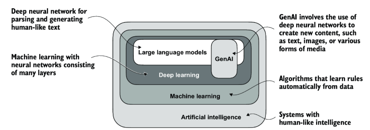
5.6 Rewriting Logistic Regression as a Neural Network
Now we observe that this model is mathematically equivalent to a one-layer neural network:
- Inputs: \(x_1, x_2, x_3, \dots\)
- One output neuron
- Sigmoid activation
- A bias term modeled as a fixed input node with value 1 and a learnable weight
See the previous section for a diagram and matrix breakdown of this equivalent neural network.
Models can be in different modes, evaluation mode.
5.6.1 Mathematical Representation
Logistic regression with a bias term can be interpreted as a neural network with:
- Input vector \(\, \tilde{x} \in \mathbb{R}^4 \,\), including a constant 1 for bias
- Weight vector \(\, \tilde{w} \in \mathbb{R}^4 \,\)
- Sigmoid activation at the output
5.6.1.1 Input vector (with bias):
\[ \tilde{x} = \begin{bmatrix} 1 \\ x_1 \\ x_2 \\ x_3 \end{bmatrix} \]
5.6.1.2 Weight vector (including bias):
\[ \tilde{w} = \begin{bmatrix} b \\ w_1 \\ w_2 \\ w_3 \end{bmatrix} \]
5.6.1.3 Linear combination:
\[ z = \tilde{w}^\top \tilde{x} = b + w_1 x_1 + w_2 x_2 + w_3 x_3 \]
5.6.1.4 Sigmoid output:
\[ \hat{y} = \sigma(z) = \frac{1}{1 + e^{-z}} \]
5.6.2 Summary Table
| Element | Symbol | Shape | Notes |
|---|---|---|---|
| Input (with bias) | \(\, \tilde{x} \,\) | \(\, \mathbb{R}^{4 \times 1} \,\) | 3 features + 1 bias |
| Weights (with bias) | \(\, \tilde{w} \,\) | \(\, \mathbb{R}^{4 \times 1} \,\) | learnable params |
| Output | \(\, \hat{y} \,\) | \(\, \mathbb{R} \,\) | scalar probability |
This is a Shinylive application embedded in a Quarto doc.
5.7 Neural Network Architectures
Today, nearly all state-of-the-art AI systems, including ChatGPT, are built around transformer architectures — which themselves rely heavily on feedforward networks as core subcomponents. However, other architectures like CNNs and RNNs continue to play crucial roles in specific areas such as computer vision and on-device speech processing.
| Architecture | Description | Common Use Cases |
|---|---|---|
| Feedforward Neural Network (FNN) | The simplest type of neural network where data flows in one direction—from input to output—through one or more hidden layers. No memory or recurrence. Often called a Multilayer Perceptron (MLP). | Image classification (with vector inputs), tabular data prediction, building blocks in LLMs (e.g., transformer feedforward layers) |
| Convolutional Neural Network (CNN) | Uses convolutional layers with local filters and shared weights to process spatial or grid-like data. Often followed by pooling layers to reduce dimensionality. | Image and video recognition, object detection, facial recognition, medical imaging |
| Recurrent Neural Network (RNN) | Designed for sequential data. Uses internal memory (hidden state) to capture dependencies across time steps. Each output depends on previous inputs. | Language modeling, time-series forecasting, speech recognition |
| Long Short-Term Memory (LSTM) / GRU | Variants of RNNs that solve the vanishing gradient problem. Maintain long-range dependencies using gated mechanisms. | Machine translation, stock price prediction, chatbot state tracking |
| Transformer | Uses self-attention to weigh relationships between tokens in a sequence. Does not rely on recurrence. Stacked layers often include self-attention + feedforward sub-layers. | Large Language Models (GPT, BERT), translation, code generation, question answering |
| Autoencoder | Learns a compressed (latent) representation of input data and reconstructs it. Composed of an encoder and decoder. Often unsupervised. | Dimensionality reduction, denoising images, anomaly detection |
| Generative Adversarial Network (GAN) | Consists of a generator and a discriminator in a game-theoretic setup. The generator creates synthetic data; the discriminator judges real vs. fake. | Image synthesis, data augmentation, deepfake generation, art creation |